The constant product formula in Uniswap v3

Our goal is to derive the constant product formula based on real reserves for a segment, given by

and from there recover some of the formulas obtained in the previous chapter.

This chapter is optional. It introduces no fundamentally new concepts compared to the previous ones, but offers a different perspective on deriving real reserves from price and liquidity. It can be skipped without any detriment to the rest of this book.

Uniswap is a Constant Product Automated Market Maker. In Uniswap v2, if we disregard fees, swaps in the pool follow the rule that the constant $k$ in the formula $xy=k$ remains unchanged, with $x$ and $y$ representing the pool’s reserves of tokens X and Y. In this sense, one can say that the formula $xy=k$ defines the behavior of swaps in the pool.

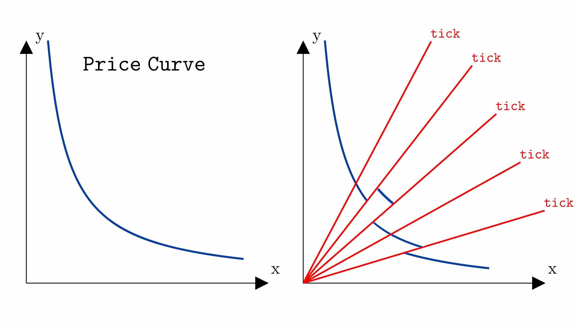
Uniswap v3 is also a Constant Product AMM, with the main difference being that the pool does not have constant liquidity but is composed of several curve segments, each with a certain liquidity $L$.

In each segment, swaps follow the same behavior as in Uniswap v2 and, disregarding fees, must maintain the value $L$ constant in the formula $L^2 = xy$, as long as the swap does not cross the boundaries of the segment.

Thus, the formula governing swaps in a segment remains $L^2 = xy$. However, unlike in Uniswap v2, $x$ and $y$ are not the segment’s real reserves but its virtual reserves, i.e., the reserves the segment would have if it extended to an infinite curve (see the chapter on real and virtual reserves).

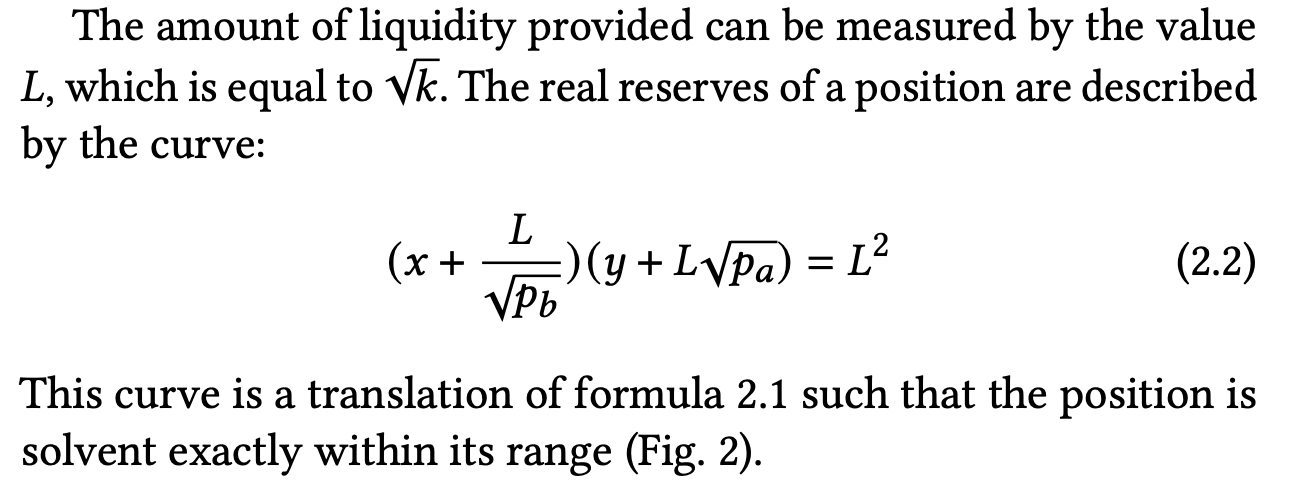
One might ask whether the constant product formula $L^2=xy$ for a segment could be expressed in terms of the segment’s real reserves rather than its virtual reserves. The answer is yes. In fact, this formula can be found on page 2 of the Uniswap v3 whitepaper, as shown below (here, $x$ and $y$ denote the real reserves, which we denote as $x_r$ and $y_r$ in our notation). This is the same formula shown in the introduction.

The formula above establishes a relationship between liquidity, segment boundaries, and real reserves. In our notation, this formula should be written as

where $p_l$ is the price at the lower tick, $p_u$ is the price at the upper tick, and $L$ is the liquidity.

For a given segment, these values are fixed, while the real reserves vary. This is similar to Uniswap v2, where liquidity $k$ is fixed in $k=xy$ and the reserves $x$ and $y$ can change. In both cases, the formulas constrain the possible reserve values—if the reserves of one token increase, the reserves of the other must decrease so that the liquidity remains constant.

This idea can be better visualized in the interactive tool below. You can choose the upper tick, lower tick, the liquidity of the segment and the current price. As the price moves, the real reserves $x_r$ and $y_r$ change, but in such a way that the liquidity $L$ stays constant. In other words, the proportion between the real reserves is not arbitrary but fully determined by the liquidity and the tick boundaries.

One major difference between v2 and v3 is that, in v3, one of the reserves can reach zero without the other approaching infinity. It’s normal to exhaust the real reserves of one token in a segment, at which point the price moves to the next segment.

It’s worth noting that the constant product formula appears nowhere in the codebase. In Uniswap v2, the protocol can simply enforce the constant product formula in swaps. In v3, however, this is more complex because the price may pass through multiple segments during a swap.

Still, the constant product formula can be used to derive expressions for the real reserves in terms of the segment boundaries, liquidity, and current price. We already derived these formulas in the previous chapter by other means, and for this reason, this chapter is optional.

Nevertheless, if the reader wishes to understand where the constant product formula comes from and how it can be used to calculate the real reserves of a segment, that is the purpose of this chapter, and we invite you to proceed.

Relating the real and virtual reserves in a segment

The constant product formula for a segment is the same as in Uniswap v2,

but now $x$ and $y$ are virtual reserves.

We can derive the constant product formula for real reserves if we find a way to relate virtual reserves to real reserves.

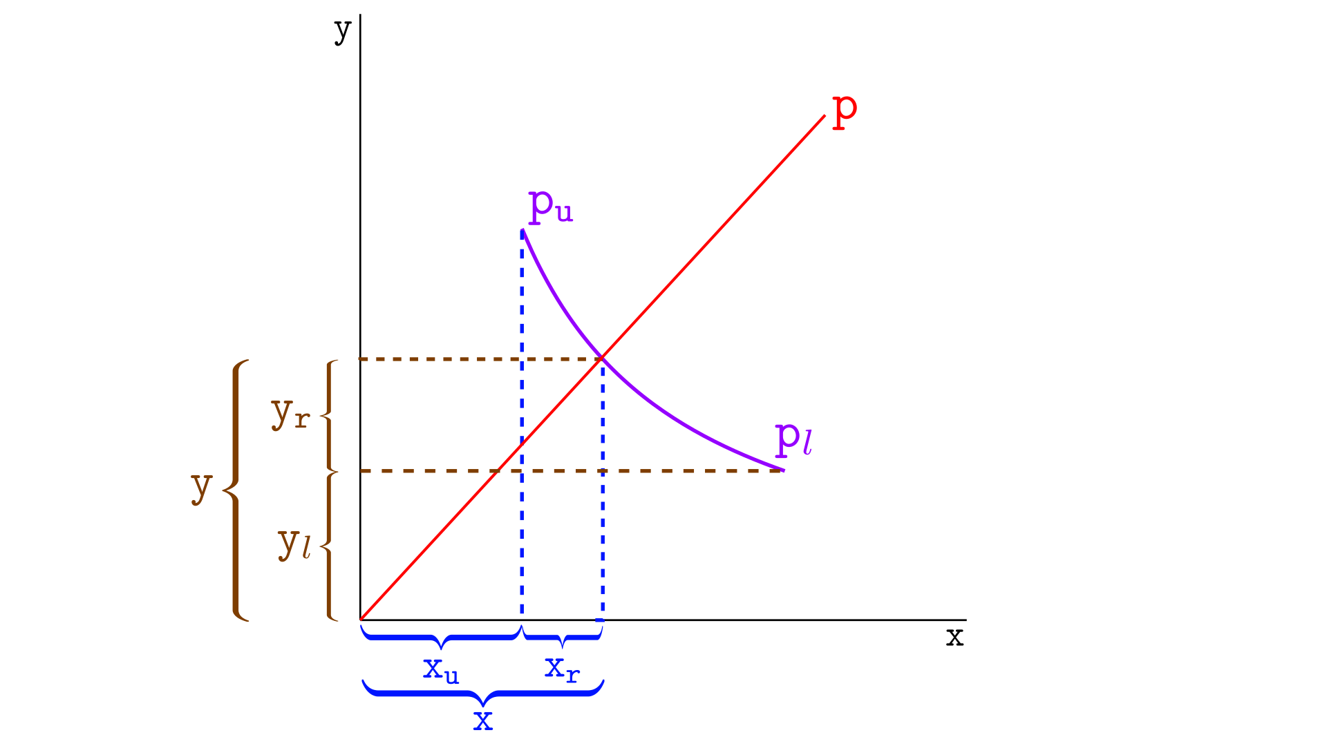
Consider the illustration below, where $p_l$ is the price at the lower tick and $p_u$ is the price at the upper tick.

In the image above, we have

• $(x,y)$ are the virtual reserves of the current price,
• $y_l$ are the virtual reserves in Y at $p_l$ - the amount of tokens Y the segment would have if it were an infinite curve and the price were at $p_l$. However, we are more interested in $y_l$ geometrically than in its interpretation,
• $x_u$ are the virtual reserves in X at $p_u$,
• $(x_r, y_r)$ are the real reserves of the segment.

The relation between virtual and real reserves is then given by

We can use these relations in $L^2=xy$, substituting $x$ and $y,$ to get

In a segment, $x_r$ and $y_r$ can vary during swaps, but $x_u$ and $y_l$ depend only on the segment boundaries, so they are constants for the segment. Thus, if we can obtain $x_u$ and $y_l$, we have found the desired formula. We derived formulas to obtain $x_u$ and $y_l$ in the previous chapter, and in the following section we will use these formulas to derive the constant product formula for real reserves.

The constant product formula for the real reserves

In the chapter on real and virtual reserves, we learned how to find the virtual reserves of a segment from price and liquidity: $x = L/\sqrt{p}$ and $y=L \sqrt{p}$. We can use these formulas to obtain $x_u$ and $y_l$ as follows:

Using these values, we can write the constant product formula

as

This formula is valid for a segment with liquidity $L$, where the lower tick is $p_l$ and the upper tick is $p_u$.

We now have a constant product formula that relates liquidity, real reserves, and segment boundaries, without any reference to virtual reserves.

Note that calculating the liquidity of a segment from the real reserves is not straightforward because the formula above involves the parameter $L$ on both sides of the equation; it is a quadratic equation in $L$.

In practice, we don’t need to worry about this because the protocol does not use the above formula to calculate liquidity. Instead, the protocol stores information about liquidity and, from the given liquidity, calculates the real reserves for tokens X and Y between two prices.

Thus, what we are interested in is finding a formula to calculate $x_r$ and $y_r$ based on the segment’s liquidity, boundaries, and the current price.

In the previous chapter, we already derived these formulas without any reference to the constant product formula—as stated in the introduction, the constant product formula is not strictly necessary for this.

For educational purposes, we will re-derive the formulas from the previous chapter using the constant product formula. The key idea is that, even though the constant product formula is not used in the codebase, the formulas for calculating real reserves based on the current price, liquidity, and the segment boundaries are indeed used by the codebase, and those formulas can be derived from the constant product formula.

To demonstrate this, let’s perform the derivation for the three possible scenarios:

1. When the current price is at or below the lower tick, so there are only real reserves in tokens X,
2. When the current price is at or above the upper tick, so there are only real reserves in tokens Y,
3. When the current price is within the segment, so there are real reserves in both tokens X and Y.

Let’s begin with the case where the current price is at or below the lower tick

1. Only tokens X in a segment

In the scenario where the segment only has X tokens, then $y_r$ equals zero and we can work out the constant product formula to derive $x_r$, as follows:

Note this is identical to the formula we derived in the last chapter.

Now let’s consider the case where the segment contains only Y tokens—when the current price is at or above the upper tick.

2. Only tokens Y in a segment

In the scenario where the segment only has Y tokens, then $x_r$ equals zero and we can work out the constant product formula to derive $y_r$, as follows:

Note this is identical to the formula we derived in the last chapter.

We now turn to the final scenario, where the price lies between the lower tick and the upper tick.

3. Both tokens in the segment

When the price is between the lower and upper ticks, the segment will have both tokens X and Y.

The constant product formula

does not involve the current price, nor can we calculate $x_r$ and $y_r$ from it alone. Note that we have two unknowns ($x_r$ and $y_r$) but only one equation. To solve this problem, we need another equation.

We know that the formula for price is $p = y/x$ in terms of virtual reserves. Thus, in terms of real reserves, we have:

Now we have two equations (the constant product formula and the price) and two unknowns ($x_r$ and $y_r$). We can rearrange the price formula as:

The term on the left-hand side appears in the constant product formula, so we can substitute it there.

Now that we have $x_r$, we can use this expression in the constant product formula to find $y_r$:

The formulas for $x_r$ and $y_r$ are identical to those we obtained in the previous chapter.

Summary

The constant product formula for a segment with liquidity $L$ between a lower tick $p_l$ and an upper tick $p_u$ is given by

where $x_r$ and $y_r$ are the real reserves in tokens X and Y.