INTT Algorithm by Hand

As seen in the previous article, the Inverse Number Theoretic Transform (INTT) is performed using a Vandermonde matrix, just like the NTT. This shows that both evaluation via the NTT and interpolation via the INTT are similar operations.

The problem with directly using the Vandermonde matrix for evaluation or interpolation is that multiplying a k×kk \times k matrix by a vector takes O(k2)\mathcal{O}(k^2) time. Fortunately, when using the kk-th roots of unity, with kk a power of 2, a fast method that does not rely on matrix multiplication can be used, reducing the time complexity to O(klogk)\mathcal{O}(k \log k).

The fast method for the NTT was introduced in the chapter “NTT Algorithm by Hand.” In this chapter, we study the fast method for the INTT.

The idea is simple: to interpret polynomial interpolation as an evaluation, allowing the use of the same method employed for the NTT.

Evaluation and Interpolation

As a recap, the NTT allows us to transform a polynomial of degree at most k1k-1 from its coefficient form,

[a0a1...ak1]\begin{bmatrix}a_0 \\ a_1 \\ ... \\ a_{k-1} \end{bmatrix}

to its point-value form,

[f(ω0)f(ω1)...f(ωk1)]\begin{bmatrix} f(\omega^0) \\ f(\omega^1) \\ ... \\ f(\omega^{k-1}) \end{bmatrix}

by evaluating the polynomial at the kk-th roots of unity. This is called evaluation.

Interpolation is the opposite of evaluation: it is the process of transforming a polynomial from its point-value form to its coefficient form.

Interpolation as evaluation

Evaluations and interpolations at the kk-th roots of unity are similar operations because both are performed using a Vandermonde matrix.

For better visualization, consider a polynomial of degree at most 3,

f(x)=a+bx+cx2+dx3,f(x) = a + bx + cx^2 + dx^3,

evaluated at the 44-th roots of unity

f(1),f(ω),f(ω2),f(ω3).f(1), f(\omega), f(\omega^{2}),f(\omega^{3}).

The evaluation can be written as

[f(1)f(ω)f(ω2)f(ω3)]=[11111ωω2ω31ω2ω4ω61ω3ω6ω9][abcd].\begin{aligned}\begin{bmatrix}f(1) \\f(\omega) \\f(\omega^2) \\f(\omega^3)\end{bmatrix}=\begin{bmatrix}1 & 1 & 1 & 1 \\1 & \omega & \omega^2 & \omega^3 \\1 & \omega^2 & \omega^4 & \omega^6 \\1 & \omega^3 & \omega^6 & \omega^9\end{bmatrix}\begin{bmatrix}a \\b \\c \\d\end{bmatrix}.\end{aligned}

The interpolation can be written as

[abcd]=14[11111ω1ω2ω31ω2ω4ω61ω3ω6ω9][f(1)f(ω)f(ω2)f(ω3)].\begin{aligned} \begin{bmatrix}a \\ b \\ c \\ d \end{bmatrix}= \frac{1}{4}\begin{bmatrix}1 & 1 & 1 & 1 \\1 & \omega^{-1} & \omega^{-2} & \omega^{-3} \\1 & \omega^{-2} & \omega^{-4} & \omega^{-6} \\1 & \omega^{-3} & \omega^{-6} & \omega^{-9}\end{bmatrix}\begin{bmatrix}f(1) \\f(\omega) \\f(\omega^2) \\f(\omega^3)\end{bmatrix}. \end{aligned}

Inspired by the evaluation structure, we can view f(1)4,f(ω)4,f(ω2)4\frac{f(1)}{4}, \frac{f(\omega)}{4}, \frac{f(\omega^2)}{4} and f(ω3)4\frac{f(\omega^3)}{4} as the coefficients of a new polynomial f~(x)\tilde{f}(x), defined as

f~(x)=14(f(1)+f(ω)x+f(ω2)x2+f(ω3)x3).\tilde{f}(x) = \frac{1}{4}\big(f(1) + f(\omega)x + f(\omega^2) x^2 + f(\omega^3) x^3\big).

In this terms, the coefficients a,b,ca,b,c and dd are the evaluations of f~(x)\tilde{f}(x) at the following points:

a=f~(1)b=f~(ω1)c=f~(ω2)d=f~(ω3)\begin{aligned} a &= \tilde{f}(1) \\ b &= \tilde{f}(\omega^{-1}) \\ c &= \tilde{f}(\omega^{-2}) \\ d &= \tilde{f}(\omega^{-3}) \\ \end{aligned}

Therefore, we can interpret interpolation as the evaluation of another polynomial. The crucial observation is that the inverse NTT does not require a fundamentally different algorithm.

Once the point-value representation is reinterpreted as the coefficient vector of a new polynomial, interpolation becomes an evaluation at a permuted set of roots of unity. In this sense, evaluation and interpolation are the same operation.

Avoiding working with inverses of the roots of unity

As shown in the transformation

[abcd]=14[11111ω1ω2ω31ω2ω4ω61ω3ω6ω9][f(1)f(ω)f(ω2)f(ω3)],\begin{aligned} \begin{bmatrix}a \\ b \\ c \\ d \end{bmatrix}= \frac{1}{4}\begin{bmatrix}1 & 1 & 1 & 1 \\1 & \omega^{-1} & \omega^{-2} & \omega^{-3} \\1 & \omega^{-2} & \omega^{-4} & \omega^{-6} \\1 & \omega^{-3} & \omega^{-6} & \omega^{-9}\end{bmatrix}\begin{bmatrix}f(1) \\f(\omega) \\f(\omega^2) \\f(\omega^3)\end{bmatrix}, \end{aligned}

the interpolation involves evaluations at the inverses of the roots of unity. However, we can avoid working with inverses.

Consider ω1\omega^{-1}. Among the 44th roots of unity, it is the element that, when multiplied by ω\omega, gives 1. Since

ωω3=ω41,\omega \cdot \omega^3 = \omega^4 \equiv 1,

we have ω1=ω3\omega^{-1} = \omega^3.

Similarly,

ω2=ω2,ω3=ω.\begin{aligned} \omega^{-2} &= \omega^2, \\ \omega^{-3} &= \omega. \end{aligned}

Thus, the coefficients a,b,ca,b,c and dd are the evaluations of

f~(x)=14(f(1)+f(ω)x+f(ω2)x2+f(ω3)x3)\tilde{f}(x) = \frac{1}{4}\big(f(1) + f(\omega)x + f(\omega^2) x^2 + f(\omega^3) x^3\big)

at the following points:

a=f~(1),b=f~(ω1)=f~(ω3),c=f~(ω2)=f~(ω2),d=f~(ω3)=f(ω).\begin{aligned} a &= \tilde{f}(1), \\ b &= \tilde{f}(\omega^{-1}) = \tilde{f}(\omega^{3}), \\ c &= \tilde{f}(\omega^{-2}) = \tilde{f}(\omega^{2}), \\ d &= \tilde{f}(\omega^{-3}) = f(\omega). \\ \end{aligned}

Using the fact that ω2=1\omega^2 = -1, we can rewrite these as

a=f~(1),b=f~(ω3)=f~(ω),c=f~(ω2)=f~(1),d=f~(ω).\begin{aligned} a &= \tilde{f}(1), \\ b &= \tilde{f}(\omega^{3}) = \tilde{f}(-\omega), \\ c &= \tilde{f}(\omega^{2}) = \tilde{f}(-1), \\ d &= \tilde{f}(\omega^{}). \\ \end{aligned}

Doing the INTT by hand

A polynomial of degree at most k1k-1, where kk is a power of 2, can be evaluated at the kk-th roots of unity using the fast method explained in the chapter NTT Algorithm by Hand.

The evaluations of

f~(x)=14(f(1)+f(ω)x+f(ω2)x2+f(ω3)x3)\tilde{f}(x) = \frac{1}{4}\big(f(1) + f(\omega)x + f(\omega^2) x^2 + f(\omega^3) x^3\big)

at the points f~(1),f~(1),f~(ω)\tilde{f}(1), \tilde{f}(-1), \tilde{f}(\omega) and f~(ω)\tilde{f}(-\omega) are illustrated below.

The idea is to group the even and odd powers as

f~(x)=14(f(1)+f(ω2)x2)+x(f(ω)+f(ω3)x2)),\tilde{f}(x) = \frac{1}{4}\big(f(1) + f(\omega^2) x^2) + x(f(\omega) + f(\omega^3) x^2)\big),

and evaluate f~(x)\tilde{f}(x) at 1\sqrt{\sqrt{1}}. At each evaluation of an innermost square root, the expression branches into two, one for each value of the square root. This continues until no square roots remain, at which point the procedure ends.
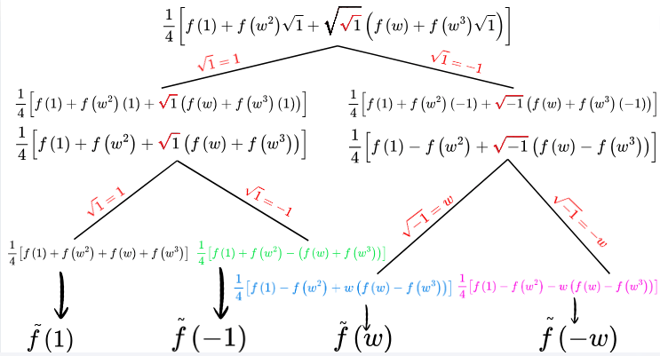
INTT by hand

We obtain

a=f~(1)=14(f(1)+f(ω)+f(ω2)+f(ω3)),b=f~(ω)=14(f(1)f(ω2)ω(f(ω)f(ω3))),c=f~(1)=14(f(1)+f(ω2)(f(ω)+f(ω3))),d=f~(ω)=14(f(1)f(ω2)+ω(f(ω)f(ω3))).\begin{aligned} a&= \tilde{f}(1) = \frac{1}{4}\big( f(1)+f(\omega)+ f(\omega^2)+f(\omega^3)\big), \\ b&= \tilde{f}(-\omega) = \frac{1}{4}\big( f(1)-f(\omega^2) - \omega( f(\omega)-f(\omega^3))\big), \\ c&= \tilde{f}(-1) = \frac{1}{4}\big( f(1)+f(\omega^2) - ( f(\omega)+f(\omega^3))\big), \\ d&= \tilde{f}(\omega) = \frac{1}{4}\big( f(1)-f(\omega^2) + \omega( f(\omega)-f(\omega^3))\big). \\\end{aligned}

Let us confirm that this matches the result obtained from the Vandermonde matrix:

[abcd]=14[11111ω1ω2ω31ω2ω4ω61ω3ω6ω9][f(1)f(ω)f(ω2)f(ω3)].\begin{aligned} \begin{bmatrix}a \\ b \\ c \\ d \end{bmatrix}= \frac{1}{4}\begin{bmatrix}1 & 1 & 1 & 1 \\1 & \omega^{-1} & \omega^{-2} & \omega^{-3} \\1 & \omega^{-2} & \omega^{-4} & \omega^{-6} \\1 & \omega^{-3} & \omega^{-6} & \omega^{-9}\end{bmatrix}\begin{bmatrix}f(1) \\f(\omega) \\f(\omega^2) \\f(\omega^3)\end{bmatrix}. \end{aligned}

Using

ω1=ω3=ω,ω2=ω2=1,ω3=ω,\begin{aligned} \omega^{-1} &= \omega^3 = - \omega, \\ \omega^{-2} &= \omega^2 = -1, \\ \omega^{-3} &= \omega, \end{aligned}

we rewrite it as

[abcd]=14[11111ω1ω11111ω1ω][f(1)f(ω)f(ω2)f(ω3)].\begin{aligned} \begin{bmatrix}a \\ b \\ c \\ d \end{bmatrix}= \frac{1}{4}\begin{bmatrix}1 & 1 & 1 & 1 \\1 & - \omega & -1 & \omega \\1 & -1 & 1 & -1 \\1 & \omega & -1 & -\omega\end{bmatrix}\begin{bmatrix}f(1) \\f(\omega) \\ f(\omega^2) \\f(\omega^3)\end{bmatrix}. \end{aligned}

This leads to

a=f~(1)  =  14(f(1)+f(ω)+f(ω2)+f(ω3)),b=f~(ω)  =  14(f(1)f(ω2)ω(f(ω)f(ω3))),c=f~(1)  =  14(f(1)+f(ω2)(f(ω)+f(ω3))),d=f~(ω)  =  14(f(1)f(ω2)+ω(f(ω)f(ω3))).\begin{alignat*}{3} a &= \tilde{f}(1) &\;=\;& \frac{1}{4}\big( f(1)+f(\omega)+ f(\omega^2)+f(\omega^3)\big), \\ b &= \tilde{f}(-\omega) &\;=\;& \frac{1}{4}\big( f(1)-f(\omega^2) - \omega( f(\omega)-f(\omega^3))\big), \\ c &= \tilde{f}(-1) &\;=\;& \frac{1}{4}\big( f(1)+f(\omega^2) - ( f(\omega)+f(\omega^3))\big), \\ d &= \tilde{f}(\omega) &\;=\;& \frac{1}{4}\big( f(1)-f(\omega^2) + \omega( f(\omega)-f(\omega^3))\big). \end{alignat*}

which are the same expressions obtained by the fast algorithm.

The key difference is that the fast algorithm runs in O(klogk)\mathcal{O}(k \log k) time, whereas the direct matrix multiplication takes O(k2)\mathcal{O}(k^2) time.

Polynomials of degree k1k-1

What we did in the previous section for a polynomial of degree 33 can be extended to polynomials of any degree.

Suppose we have a polynomial f(x)f(x) evaluated at the kk-th roots of unity, where kk is a power of 22:

f(ω0),f(ω1),f(ω2),...,f(ωk1)f(\omega^0), f(\omega^1), f(\omega^2), ..., f(\omega^{k-1})

To recover the coefficients of the polynomial f(x)f(x), of degree at most k1k-1, that passes through these points, we define a new polynomial f~(x)\tilde{f}(x) as

f~(x)=1k(f(1)+f(ω)x+f(ω2)x2+...+f(ωk1)xk1)\tilde{f}(x) = \frac{1}{k}\big(f(1) + f(\omega)x + f(\omega^2) x^2 + ...+ f(\omega^{k-1}) x^{k-1}\big)

The coefficients of f(x)f(x) are then given by

a0=f~(ω0)a1=f~(ω1)=f~(ωk1)a2=f~(ω2)=f~(ωk2)...ak1=f~(ω(k1))=f~(ω1)\begin{aligned} a_0 &= \tilde{f}(\omega^0) \\ a_1 &= \tilde{f}(\omega^{-1}) = \tilde{f}(\omega^{k-1}) \\ a_2 &= \tilde{f}(\omega^{-2}) = \tilde{f}(\omega^{k-2}) \\ ... \\ a_{k-1} &= \tilde{f}(\omega^{-(k-1)}) = \tilde{f}(\omega^{1}) \\ \end{aligned}

This article is part of a series on the Number Theoretic Transform in our ZK Book

Ready to Get Started?Join Thousands of Users Today

Start your free trial now and experience the difference. No credit card required.

© 2026 Better-Start. All rights reserved.